MS-Excel: Create Result or Grade using VLOOKUP function

You can create a result average or division/ gradation system using Sum and IF function, today We will discuss that how to create a Grade system result using VLOOKUP function in Ms-Excel.

Software Requirement:

• Here I’m using Microsoft Office Home and student 2019, You may use any upper/ lower version as well.

Knowledge: If you are familiar with basic Excel uses then you can easily understand this function.

Let’s begin

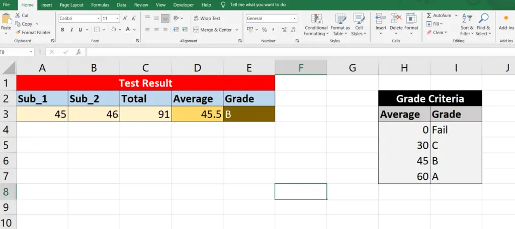
here in this above image as you can see that i’ve already made a design from A1: E3 (Result Design) and H2:I7) Grade criteria List- Now do step by step as below…

Steps:

• 1st Create Test Result design like below

• Now Do the Total and Average formula as below

Total Formula:

Average Formula:

• Before Writing the Grade formula you must have to prepare the Gradation system List as first image
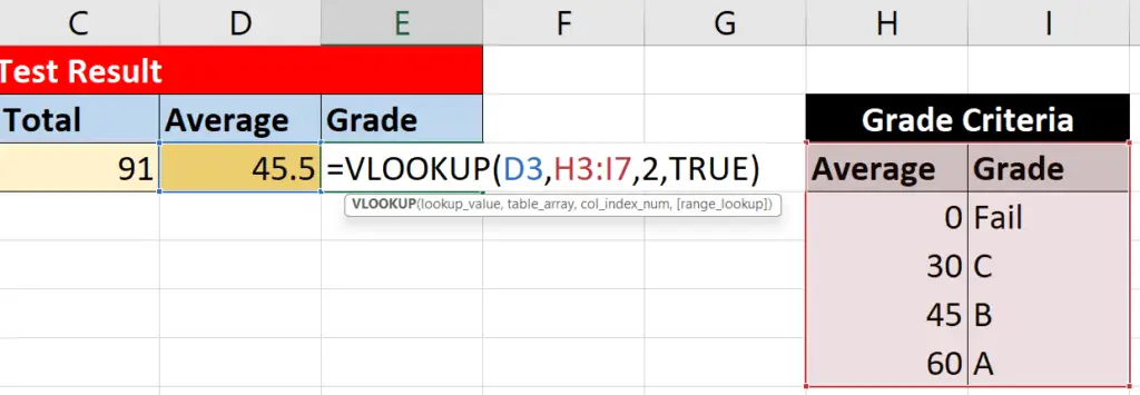
• Now Select Grade Cell and Write this formula
• =VLOOKUP(Average Cell, Grade Criteria Cells (H3:I7), 2, True)

• Press ENTER key
• Now change the Subject’s number and check the formula is working or not.

Thank you, If you like this solution then please write your valuable feedback…